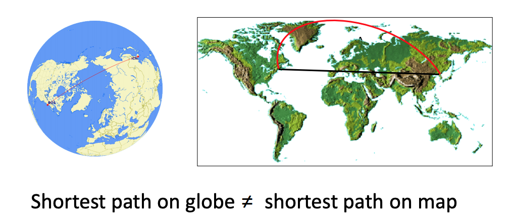
In machine learning and robotics, data and model parameters often lie on spaces which are non-Euclidean. This means that these spaces don’t follow the flat Euclidean geometry and our models and algorithms need to account for this. To clarify this using a well-known example, let’s say our optimization algorithm gave us an update to apply onto the parameter space which we wrongly assumed is Euclidean, but was actually elliptical. This is the case shown below when minimizing the distance between two points on the earth’s surface. If we optimized in the Euclidean space, we would end up with the flat, straight line shown in black, whereas we know that the shortest path between the two points (the geodesic) would in reality be the red line due to the elliptical geometry of the earth (that’s why flight routes appear curved on 2D maps). This example shows why it’s important to correctly model the geometry of the parameter space during optimization. This post will introduce the concept of a manifold, motivate the need to do optimization over them in machine learning and finally go into some detail about doing this optimization for Matrix Lie groups like rotation matrices and poses which frequently come up in robotics and computer vision.

What is a manifold

Intuitively, a manifold is a topological space that locally looks like a Euclidean space. For example, the earth’s surface is spherical but looks planar locally. Stated more formally, each point on an n-dimensional manifold has a local neighbourhood that is homeomorphic (one-to-one mapping with a continuous inverse function) to the Euclidean space of n dimensions. An even more formal definition based on Hausdorff spaces can be found in this blog which does a really good job at giving an introduction to these concepts. For those who understand better from video lectures, I found these short, but very lucid explanations on this YouTube Channel. For this blog post, the above intuitive definition of a space that can be deformed locally to be Euclidean should be sufficient.

Why care about manifolds in machine learning

As mentioned earlier, we often make Euclidean assumptions about our data or models which might not be correct. For example, representing a document as a vector in Euclidean space might be problematic as algebraic operations like addition or multiplication with a scalar on these data points might not have any meaning in data space. Another example in computer vision [¹] is representing images using a low dimensional subspace explicitly assuming that these points lie on a Grassmann Manifold. Many other manifold learning methods like LLE (Locally Linear Embedding) [²] and Isomap [³] try to do the same without explicitly defining a manifold of choice. This is a direct motivation of the extensively used manifold hypothesis in machine learning. This more optimal and compact representation can then be used for various learning-based estimation tasks and better feature learning. There are tons of other examples where manifolds are useful for optimization with different data types ranging from trajectories for path planning in robotics to graphs for gene expressions in genetics to 3D shapes and surfaces in computer vision, all of which involve a non-Euclidean manifold.

Optimization on Lie Groups

Modeling rotations is a very useful task in computer vision, graphics and robotics. Images and their parts can be described as transformations involving rotation, motion of complicated surfaces and rigid bodies can be described using rotations and robots need to know the position and orientation of the sensors on it which again involve rotations. There are various ways to parameterize rotations when optimizing over them. A common use-case is using a $3 \times 3$ rotation matrix and running optimization algorithms to recover the real rotation values. However, when optimizing these parameters, often a gradient-based update is applied to the initial value of the rotations and these updates can modify the matrix such that it isn’t a valid rotation matrix anymore. Thus, there is a need to apply these updates on a manifold which preserves the property of the model parameters, ie the parameters continue to lie on the rotation manifold. This manifold is actually a smooth and differentiable manifold which is also called the Special Orthogonal Group or $SO(n)$ group. For 2D and 3D rotations, this is referred to as the $SO(2)$ and $SO(3)$ group respectively. These $SO(n)$ groups are a part of much broader Lie Groups which intuitively are groups allowing smooth and continuous operations on its elements (such that we can use differentiable calculus with them). Another example is the $SE(n)$ group or the Special Euclidean Group which consist of a set of rotations and translations applied simultaneously and is heavily used for rigid transformations in robotics (a robot pose ie, position and orientation is specified using this group). Essentially, using Lie Groups like $SO(n)$ or $SE(n)$ allows us to optimize over the rotations/poses in a space where they continue to lie on the rotation/pose manifold after the update is applied.

Optimizing rotations using exponential maps: The theory

This subsection will simply outline the use of exponential maps for adding rotations without going into any proofs or justifications. The next subsection talks about the intuition for our choices.

Let $R \in \mathbb{R}^{3 \times 3}$ be the initial estimate of the rotation matrix. If we add an arbitrary update matrix to it, the final matrix will almost never lie on a $SO(3)$ manifold (one straightforward way to see this is that adding arbitrary elements removes the orthogonality of the newly formed matrix).

Since rotations have 3 degrees of freedom, let $\omega \in \mathbb{R}^3$ be the update which needs to be added to the initial rotation. This vector space is also called the tangent space and is loosely the same as the something called Lie algebra or $so(3)$ of the group (a bijective mapping exists between Lie algebra and the tangent space). In order to solve the problem of doing optimizations on the rotation manifold we need a mapping which can take us from the tangent space (a vector of 3 elements) to a valid rotation lying on the $SO(3)$ manifold. This mapping from the tangent space (or in turn Lie algebra) to the Lie Group (or the manifold) is the called the exponential map. Let g be the Lie algebra and G be the Lie Group. Then the exponential map defines a mapping $g \rightarrow G$.

Since we need to apply an update on top of an initial rotation estimate while staying on its manifold, the exponential map should be able to characterize the local neighbourhood on the manifold. More specifically, we need derivatives of how the $SO(3)$ manifold changes around a specific point in order to guide how to map an arbitrary 3-vector to a valid rotation on $SO(3)$. This is done using the tangent on the points on $SO(3)$ at identity, which is the reason why its called the tangent space in the first place. The bijective mapping from $\mathbb{R}^3$ to $so(3)$ is the skew-symmetric matrix operator and the exponential map function is the matrix exponentiation function. We will come back to see why these choices make sense. For now, the figure below visually shows the mappings from $\mathbb{R}^3 \rightarrow so(3) \rightarrow SO(3)$ (image taken from the amazing course of Geometry-based Methods in Vision from CMU:

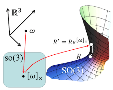
Therefore, the exponential map takes a vector from the Euclidean space and maps it to a valid rotation on the manifold.

Mathematically, for adding the update to our initial rotation, we are finding an incremental rotation $R_{inc}$ around the identity matrix and composing our initial rotation with it to get the updated rotation $R'$.

$$ \begin{align} R + \omega \triangleq R' = R . R_{inc}(\omega)\\ \end{align} $$

Here, the incremental rotation is the exponential map function shown in the figure above.

$$ \begin{align} R' = R e^{[\omega]_{\times})} \end{align} $$

where $[\omega]_{\times}$ is the skew-symmetric matrix associated with the vector $\omega$, defined as:

$$ \begin{align} [\omega]_{\times} = \begin{bmatrix} 0 & -\omega & \omega\\ \omega & 0 & -\omega\\ -\omega & \omega & 0\end{bmatrix}\\ \end{align} $$

Intuition behind exponential maps

Why does exponentiating a skew-symmetric version of the 3-vector give us a valid rotation on the $SO(3)$ manifold? This is actually a two part question. Firstly, why does $\mathbb{R}^3 \rightarrow so(3)$ mapping involve creating a skew-symmetric matrix from the vectors and secondly, why does the mapping $so(3) \rightarrow SO(3)$ involve taking matrix exponentials. The answers to these arise from the very definitions of $so(3)$ and $SO(3)$ spaces.

The skew-symmetric matrix when written in the cross product form shows that it forms the tangent for any vector $a$

$$ \begin{align} [\omega]_{\times}a = \omega \times a \quad \forall a \in \mathbb{R^3} \end{align} $$

Now, since $so(3)$ is the Lie algebra which is defined as the tangent space at identity, cross product operation and in turn the set of all skew-symmetric matrices form the so(3) space. A proof with equations is given here.

Coming to the second mapping, we can see why exponentiation leads to a valid $SO(3)$ point by analyzing the Taylor expansion of the exponential function.

$$ \begin{align} e^A = \lim_{n\to\infty} (I + \frac{1}{n} A)^n \end{align} $$

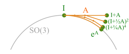
As the identity matrix is an element of the $SO(3)$ group, the term $I + \frac{1}{n} A$ becomes $SO(3)$ as $n$ tends towards infinity. Additionally raising this term to the power of $n$ also keeps this within the $SO(3)$ as the group is closed under multiplication. Another intuitive way to see this is that the first two terms of the expansion are simply $I + A$ which is what we originally (and naively) wanted to do with simple addition of rotations, but which would’ve deviated the final result from the rotation manifold. However, each additional higher power term in the expansion pulls the point towards the $SO(3)$ manifold. This can be seen in the figure below taken from Tom Drummond’s notes.

A more mathematical interpretation of exponential map is due to the fact that the exponentiation is the solution to the differential equation $\frac{dR}{dt} = AR$ which gives $R(t) = e^{tA}$. This solution creates a relation between the derivatives of the rotations and the rotations or equivalently, a relation between $so(3)$ and $SO(3)$.

It is important to note that the exponential map is an exact mapping even for arbitrarily large vectors $\omega$ and not just an approximation. Also, there is a closed form solution of the matrix exponential function for $SO(3)$ which is called Rodrigues’ Formula which makes computing these updates to the rotations pretty convenient.

Optimization over other general manifolds

In addition to the $SO(3)$, we can use similar machinery to add elements of any General Linear Groups or $GL(n)$ which are essentially the set of all $n \times n$ non-invertible matrices. All of them entail the use of exponential coordinates, but use different forms of Lie algebra depending on the group structure. In fact, even arbitrary manifolds which do not have the group structure can be optimized on through something called retractions which also maps the local coordinates onto the manifold much like the incremental rotations mentioned above. The book by Absil et al [⁴] goes into a lot of detail about optimization methods for matrix manifolds and is a great resource for any of the topics mentioned in this post.

References