Few days ago, while reading about variational autoencoders, I came to know that variational inference was in fact a generalization of the popular algorithm, expectation maximization (EM). The aim of writing this post is to explain the relationship between these two popular techniques. The post assumes the reader is familiar with the EM algorithm, but if you need a reference for it before starting here, have a look at this.

Notation

• X denotes the observed random variables
• p(X) or q(X) denotes probability distribution over the variables X
• Z denotes the latent random variables

Expectation Maximization

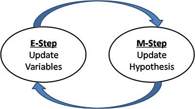
EM is used to estimate the maximum likelihood of data given the model parameters in cases where the data has some latent variables. In order to do so, EM repeats the following two steps until convergence:

E step: Estimate the latent variables according to posterior distribution calculated with the model parameters
M step: Update the model parameters by maximizing the likelihood

What this means mathematically is:

E step: Estimate $Q(\theta, \theta_t)$ for iteration $t$
M step: Maximize $Q(\theta, \theta_t)$ wrt to $\theta$

where

$$Q(\theta, \theta_t) = \mathbb E_{p(Z \mid X)}[\log p(X,Z;\theta)]$$

and the probability distribution $p$ is parameterized by $\theta$, ie $\theta$ is the model parameter.

Variational Inference

Variational inference is a method which tries to do inference in complicated graphical models where the distribution to be computed is intractable. It does this by re-framing the inference problem into an optimization problem. In the Bayesian framework, inference is formulated as computing the posterior distribution over the set of latent variables:

$$p(Z \mid X;\theta) = \frac{p(X,Z;\theta)}{\int_Z p(X,Z;\theta)}$$

The integral in the denominator is intractable for a lot of distributions of interest. So, the problem boils down to finding close approximations for it. There are sampling based techniques like MCMC which do this by constructing a Markov chain with the latent variables, but they are very slow to converge. Instead, what VI does is replace the intractable distribution, $p(Z \mid X;\theta)$ by a proxy distribution, $q(Z)$ and perform inference on it. For this to work out, the following needs to be taken care of:

1. The proxy distribution should closely resemble the original posterior
2. The proxy distribution should be simple enough to perform inference on

For measuring deviation from the posterior, we use the KL divergence of the proxy distribution with respect to the original posterior. For simplicity, I drop the model parameter $\theta$ for now, but will include it in the end.

$$ \begin{align} KL(q(Z)||p(Z \mid X)) & = \mathbb E_{q(Z)}[\log \frac{q(Z)}{p(Z \mid X)}]\\ & = \mathbb E_{q(Z)}[\log q(Z)] - \mathbb E_{q(Z)}[\log p(Z \mid X)]\\ & = \mathbb E_{q(Z)}[\log q(Z)] - \mathbb E_{q(Z)}[\log p(X,Z)] + \log(p(X))\tag{1}\\ \end{align} $$

Now, we take a detour to calculate the log likelihood for the observed data. This quantity is of interest to us because we often use it for maximum likelihood estimation.

$$\log(p(X)) = \log(\int_Z p(X,Z))$$

This is just the marginal distribution over the latent variables. Now, to change it into expectation form, we apply a small trick. We multiply and divide the term inside the integral by $q(Z)$.

$$ \begin{align} \log(p(X)) & = \log(\int_Z \frac{p(X,Z) q(Z)}{q(Z)})\\ & = \log(\mathbb E_{q(Z)}[\frac{p(X,Z)}{q(Z)}]) \end{align} $$

Now using Jensen’s Inequality, we switch the log and the expectation and update the inequality.

$$ \begin{align} \log(p(X)) & \ge \mathbb E_{q(Z)}[\log(\frac{p(X,Z)}{q(Z)})]\\ & \ge \mathbb E_{q(Z)}[\log(p(X,Z)] - E_{q(Z)}[\log(q(Z))]\tag{2}\\ \end{align} $$

The important thing to notice here is that equation $2$ places a lower bound on the log probability of the data and hence it is often called the evidence lower bound or ELBO.

Now, we go back to our equation $1$ and find that the RHS of both equations have the common term ELBO. In fact, substituting ELBO in the first equation gives us:

$$KL(q(Z)||p(Z \mid X)) = -ELBO + \log(p(X))\tag{3}$$

Finally, coming back to our original problem of minimizing the KL divergence, we can see that since the second term on the RHS of equation $3$ is independent of $q$, minimizing the KL divergence is the same as maximizing the ELBO. Furthermore, we also have seen that the log probability of the data has a lower bound called ELBO and the gap between them is quantified by the KL divergence term between the approximating distribution and the original posterior.

EM as a special case of Variational Inference

So, variational inference is all about changing the posterior estimation problem to an optimization problem, namely the maximization of ELBO. Let’s have a closer look at it, this time with the model parameters.

$$ELBO(q,\theta) = E_{q(Z)}[\log(p(X,Z;\theta)] - E_{q(Z)}[\log(q(Z))]\tag{4}$$

The ELBO in fact is a function of the probability distribution $q$ and model parameters $\theta$

The EM algorithm described in the beginning can be interpreted as an iterative algorithm of optimizing $ELBO(q,\theta)$, keeping one parameter constant at a time.

The two steps can be re-stated more generally in the following manner:

E step:

$$\mathop{\arg\,\max}\limits_q (ELBO(q,\theta_t))$$

This step does coordinate ascent on $ELBO(q,\theta_t)$ at iteration $t$.
Since we know that the optimal $q$ for the above problem will occur when the approximate distribution equals the original posterior, the solution to the above problem trivially becomes

$$q_t(Z) = p(Z \mid X)\tag{5}$$

Note that this step is the same as estimating the function $Q(\theta,\theta_t)$ as done in the E-step of EM described above. It assumes that the approximating distribution is the same as the posterior.

M step:

$$\mathop{\arg\,\max}\limits_\theta (ELBO(q_t,\theta))$$

Substituting the ELBO value from equation $4$ and substituting the E step value from equation $5$, we have

$$\mathop{\arg\,\max}\limits_\theta (E_{p(Z \mid X)}[\log(p(X,Z;\theta)] - E_{p(Z \mid X)}[\log(p(Z \mid X))])$$

Since the second expectation term is independent of $\theta$, the problem simplifies to the original M-step of the EM algorithm as described above.

$$\mathop{\arg\,\max}\limits_\theta (E_{p(Z \mid X)}[\log(p(X,Z;\theta)])$$

Conclusion

The above analysis shows that variational inference is expectation maximization when the variational distribution of VI is the same as the original posterior distribution. This means that EM assumes that the expectation over the posterior is computable and can be dealt with without any approximations and hence the KL divergence from equation $3$ becomes zero.

I highly recommend reading this review paper and these slides for more on variational inference.